(posting this to share with a few interested people)

tl;dr:

I trained a simple model on a task of pure memorization – learning a completely randomized table of bits. I experimented with limiting the dimensions to force some computation in superposition behaviour.

I found it was able to fully solve the task, and the solved solution is fairly spread across all neurons. I found a framing of the problem which makes it similar to matrix decomposition algorithms like SVD or matrix sketching, but wasn’t able to fully characterize things.

I found that for a reasonable range of parameters, the model seems to be able to learn about 2 bits per parameter. The best constructions I found could only do 1.58 bits, so I cannot explain exactly how it works.

Setup

I train a model that takes two input tokens which can each take one of \(m\) values, embeds them both in a \(d_{model}\) space, and passes the sum to a \(d_{hidden}\) neuron MLP, which outputs logits predicting two classes, 0, 1.

At the start of training, a target matrix of size \(m\times m\) is randomly generated with values \(\{0, 1\}\), and the model trained for cross entropy for each pair of inputs predicting one entry of the target. Each batch consists of the full \(m^2\) possible pairs with no sampling.

I experimented with several different embeddings:

• Trained – the embedding is trained with the rest of the model
• Random – Random Gaussian init, then normalized
• Optimized – As random, but then it is trained (separately to the model itself) to maximize orthogonality
• Basis – Sets \(d_{model}=2m\) and assigns every token a unique basis vector so they are fully orthogonal.

This model is motivated by the common example used in LLMs of investigating how they answer “Michael Jordan plays the sport of ___”. It’s been mostly established (e.g. in Fact Finding) that earlier layers find a direction corresponding to the entity “Michael Jordan”, and another for the query “plays sport?”, and moves both to the last token. Then something happens in the MLP layers to produce the answer. This toy model omits all the circuitry preceeding the final token, and assumes that only a single layer is necessary (I believe multiple layers are involved just to increase the neuron count available, and there’s no significant interaction between these recall layers). So the pair of inputs are proxies for entities (like “Michael Jordan” and properties like “plays sport”, “age” etc.

The toy model uses only two output classes for simplicity, but multiple output classes is easy to image working similarly. I also use a “total” target (every possible pair of inputs has an answer, and is trained for), but I expect similar results for partial targets which need a large enough fraction of pairs answered.

Results

Trained embeddings behaved a bit differently, I’ll skip discussing those.

Optimized behaved near identically to Random.

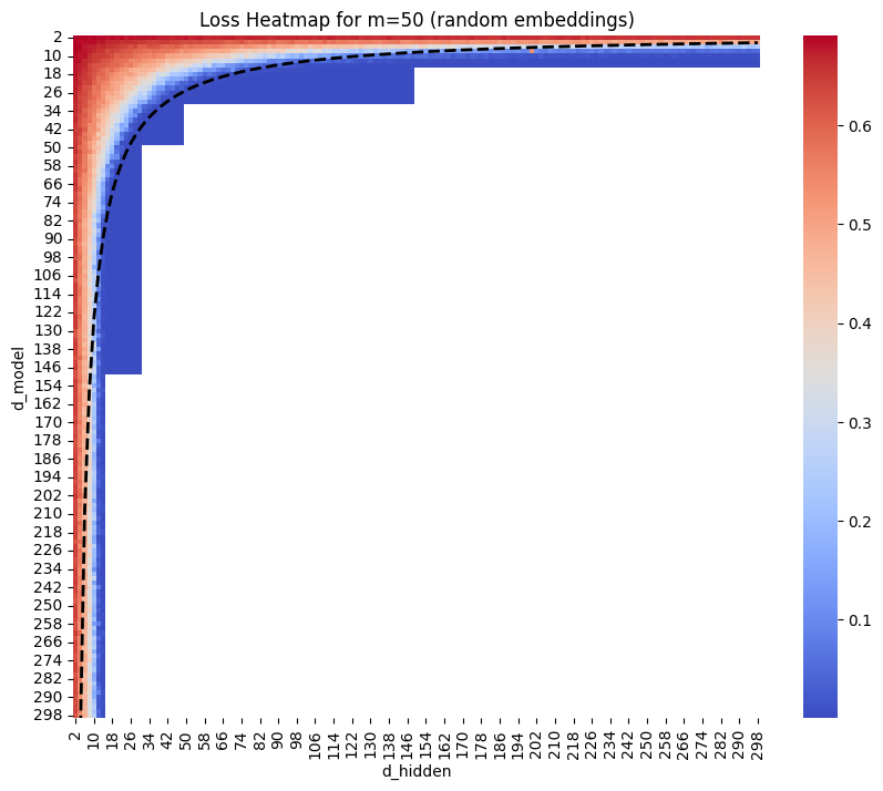
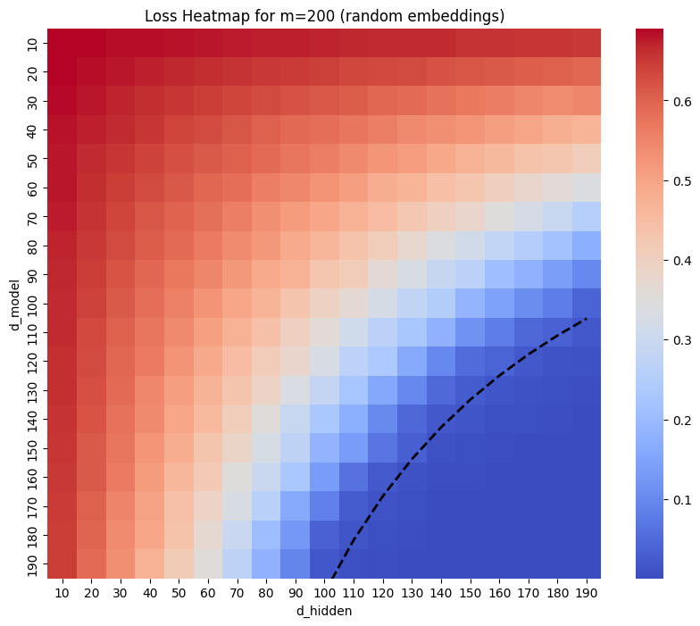
For Random embeddings, I found that in the “sweetspot” of \(d_{model}\approx d_{hidden}\) I found that loss reached zero when the number of parameters was approximately \(m^2/2\).

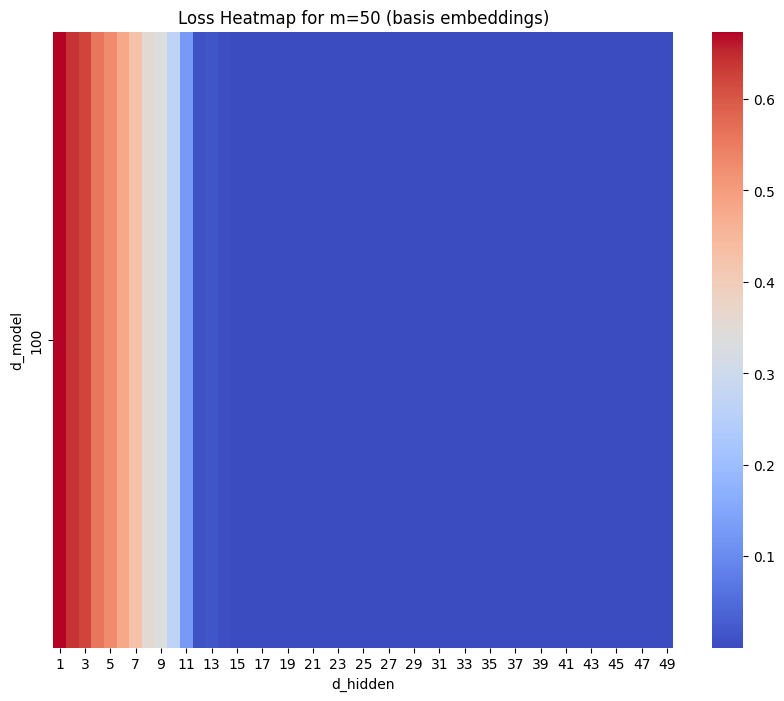
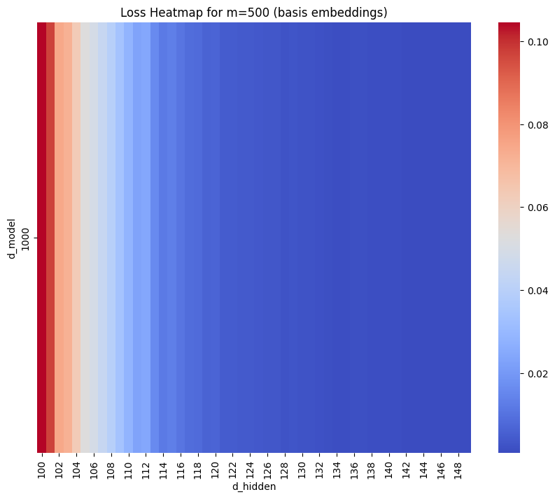
The Basis model performed similarly – (though it’s only a 1d plot as \(d_{model}\) is fixed).

Analysis

I’m unable to explain the specifics of the performance, but I did find a framing of the problem that is useful. Let’s focus on the Basis setting, where each token is fully orthogonal and there is no superposition to deal with. That means the full calculation is

\[ h = \operatorname{ReLU}(W(e_a + e_b) + c) \]

\[ \hat{y} = Rh+c’ \]

for \(a\) and \(b\) the two input tokens (indexed so that \(a\) and \(b\) are disjoint). Or we can remove the disjoint fiddliness by splitting W into two matrices

\[ h = \operatorname{ReLU}(We_a + W’e_b + c) \]

\[ h_i = \operatorname{ReLU}(W_{ia} + W’_{ib} + c_i) \]

The best way to view this is as a 2d array indexed on a and b. I illustrate with a constructed solution.

Suppose the target array is \([[1, 1, 1], [0, 1, 0], [1, 0, 1]] \).

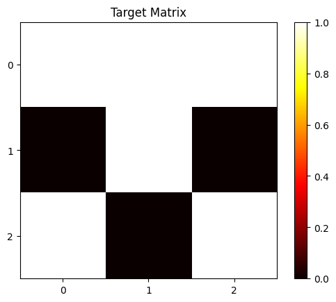
A constructed solution to this in two neurons would look like:

\[ W_0 = [1, 0, 1] , W’_0 = [1, 0, 1], c_0 = -1 \]

Which gives neuron 0 activation of

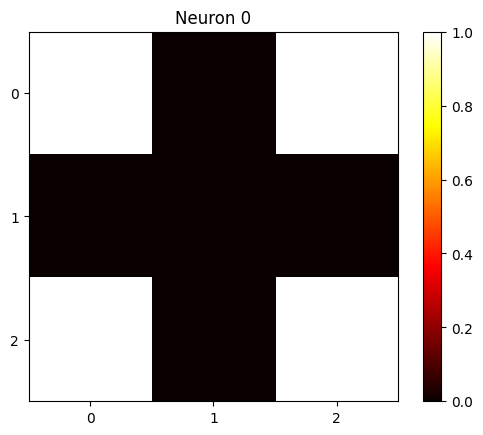
And

\[ W_1 = [1, 1, 0] W’_1 = [0, 1, 0], c_1 = -1 \]

which gives neuron 1 activation of

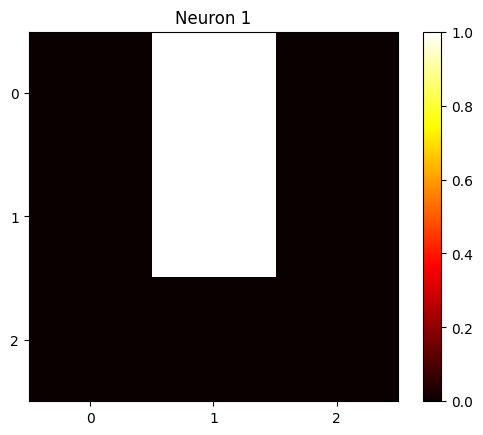
The second layer can simply sum these things together to reconstruct the output, and trivially convert to logits.

In other words, you can view the solution as a matrix decomposition of the target matrix. Each neuron contributes a rank-1 matrix to the solution, which are summed together to give the final output.

When I inspect the model, it’s messier than this as it’s free to use floating point values, and it can subtract neurons as well as add them. And other choices of basis mean the neuron matrix is not strictly rank-1, though each neuron is fully specified by \(2m+O(1)\) parameters so it is fairly deficient.

But I think it’s essentially a similar story – each neuron contributes a constrained matrix, which together sum to the target.

Using a superposition basis (\(d_{model}<2m\)) doesn’t really change this, there is a whole numerical analysis technique called “sketching” which is about how matrices can be well approximated by a smaller matrix paired with a set of random vectors. It has a similar J-L Lemma justification to feature superposition.