How to create a sharp mesh from a function without even trying
In part 1 and part 2 of the series, we looked at the Marching Cubes algorithm, and how it can turn any function into a grid based mesh. In this article we’ll look at some of the shortcomings and how we can do better.
Marching Cubes is easy to implement, and therefore ubiquitous. But it has a number of problems:
- Complexity
Even though you only need process one cube at a time, Marching Cubes ends up pretty complicated as there are a lot of different possible cases to consider.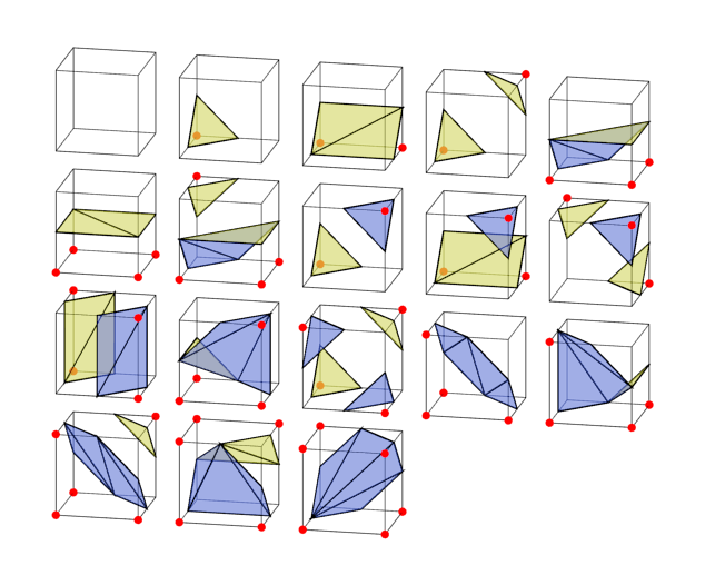
- Ambiguity
Some cases in Marching Cubes cannot be obviously resolved one way or another. In 2d, if you have two opposing corners, it’s impossible to say if they are meant to be joined or not.In 3d, the problem is even worse, as inconsistent choices can leave you with a leaky mesh. We had to write extra code to deal with that in part 2.
- Marching Cubes cannot do sharp edges and corners
Here’s a square approximated with Marching Cubes.The corners have been sliced off. Adaptivity cannot help here – Marching Squares always creates straight lines on the interior of any cell, which is where the target square corner happens to lie.
So, what do do next?
Enter Dual Contouring
Dual Contouring solves these problems, and is more extensible to boot. The trade off is we need to know even more information about \( f(x) \), the function determining what is solid and what is not. Not only do we need to know the value of \( f(x) \), we also need to know the gradient \( f'(x) \). That extra information will improve the adaptivity from marching cubes.
Dual Contouring works by placing a single vertex in each cell, and then “joining the dots” to form the full mesh. Dots are joined across every edge that has a sign change, just like in marching cubes.
The “dual” in the name comes from the fact that cells in the grid becomes vertices in the mesh, which relates to the dual graph.
Unlike Marching Cubes, we cannot evaluate cells independently. We must consider adjacent ones to “join the dots” and find the full mesh. But in fact, it’s a lot simpler algorithm than Marching Cubes because there are not a lot of distinct cases. You simply find every edge with a sign change, and connect the vertices for the cells adjacent to that edge.
Gradients
The gradient of a function f is a measure of how quickly the value of f changes at a given point when moving in any given direction. It’s normally given as pair of numbers for every point, indicating how much the function changes when moving along the x-axis or y-axis.
In marching cubes, we just needed to evaluate the function \( f \) on a grid. Now, we need gradient information, and not just on the grid points, but at certain points in between as well. While there are a number of sources of this information, by far the simplest is to start with a function \( f \) that can evaluated in any point in space. We can then calculate the gradient information using calculus, or numerically. Note that the gradient is often called the normal, or hermite data, which are similar concepts.
Getting the gradient
In our simple example of a 2d circle of radius 2.5, \( f \) is defined as:
\[ f(x, y) = 2.5 – \sqrt{x^2 + y^2} \]
(in other words, 2.5 minus the distance from the origin)
With a bit of calculus, we can compute the gradient at any given position:
\[ f'(x, y) = \text{Vec2}\left(\frac{-x}{\sqrt{x^2 + y^2}}, \frac{-y}{\sqrt{x^2 + y^2}} \right) \]
But you don’t need complicated maths to get the gradient function. You can just measure the change in \( f \) when \( x \) and \( y \) are perturbed by a small amount \( d \).
\[ f'(x, y) \approx \text{Vec2}\left(\frac{f(x+d, y) – f(x-d, y)}{2d}, \frac{f(x, y+d) – f(x, y-d)}{2d} \right) \]
This works for any sufficiently smooth \( f \), providing you pick \( d \) small enough. In practice, even functions with sharp points are sufficiently smooth, as you don’t need evaluate the gradient near the sharp parts for it to work. Link to code .
Adaptivity
So far, we’ve just got the same sort of stepped look that Marching Cubes had. We need to add some adaptivity. For Marching Cubes, we chose where along the edge put a vertex. Now we have a free choice of anywhere in the interior of the cell.
First, we’ll evaluate \( f \) at each corner of the cell, and estimate where the boundary intersects each edge, i.e. the locations that would be used for vertices of marching cubes.
But instead, we load gradient information for those points. The dual contouring vertices will be placed at the point inside the cell that is most consistent with those gradients.
By picking the illustrated point, we ensure that the output faces from this cell conform as well as possible to the normals:
In practice, not all the normals around the cell are going to agree. We need to pick the point of best fit. I discuss how to handle picking that point in a later section.
Going 3d
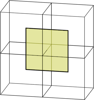
The 2d and 3d cases aren’t really that different. A cell is now a cube, not a square. And we are outputting faces, not edges. But that’s it. The routine for picking a single point per cell is the same. And we still find edges with a sign change, and then connect the points of adjacent cells, but now that is 4 cells, giving us a 4-sided polygon:
Results
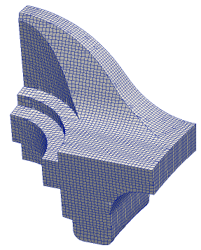
Dual contouring has a more natural look and flow to it than marching cubes, as you can see in this sphere constructed with it:
In 3d, this procedure is robust enough to pick points running along the edge of a sharp feature, and to pick out corners where they occur.
Choosing a vertex location
One major problem I glossed over before is how to choose the point location when the normals don’t point to a consistent location.
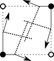
The problem is even worse in 3d when there are likely to be a lot of normals.
The way to solve this is to pick the point that is mutually the best for all the normals.
First, for each normal, we assign a penalty to locations further away from ideal. Then we sum up all the penalty functions, which will give an ellipse shaped penalty. Finally, we pick the point with the lowest penalty.
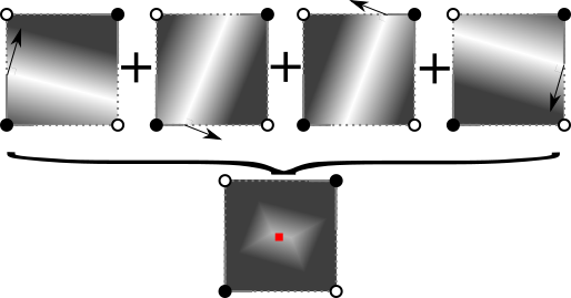
Mathematically, the individual penalty functions are the square of the distance from the ideal line for that normal. The sum of all those squared terms is a quadratic function, so the total penalty function is called the QEF (quadratic error function). Finding the minimal point of a quadratic function is a standard routine available in most matrix libraries.
In my python implementation , I use numpy’s lstsq function.
Problems
Colinear normals
Most tutorials would stop here but it’s a dirty secret that solving the QEF as described in the original Dual Contouring paper doesn’t actually work very well.
If you solve the QEF, you can find the point that is most consistent with the normals of the function. But there’s no actual guarantee that the resulting point is inside the cell.
In fact, it’s quite common for it not to be if you have large flat surfaces. In that case all the sampled normals are the same or very close, as in this diagram.
I’ve seen a lot of advice dealing with this particular problem. Several people have given up on using the gradient information, instead taking the center of the cell, or average of the boundary positions. This is called Surface Nets, and it at least has simplicity going for it.
But what I’d recommend based on my own experiments is the combination of two techniques.
Technique 1: Constrained QEF solving
Recall we were finding the cell point by finding the point that minimized the value of a given function, called the QEF. With some small changes, we can find the minimizing point within the cell.
Technique 2: Biasing the QEF
We can add any quadratic function we like to the QEF and we get another quadratic function which is still solvable. So I add a quadratic which has a minimal point in the center of the cell.
This has the effect of pulling the solution of the overall QEF towards the center.
In fact, it has a stronger effect when the normals are colinear and likely to give screwy results, while it barely affects the positions for the good case.
Using both techniques is somewhat redundant, but I think it gives the best visual results.
Better details on both techniques are demonstrated in the code .
Self interesctions
Another dual contouring annoyance is it can sometimes generate a 3d surface that intersects itself. For most uses, this is completely ignorable, so I have not addressed it.
There is a paper discussing how to deal with it: “Intersection-free Contouring on An Octree Grid” Ju and Udeshi 2006
Manifolds
While a dual contouring mesh is always water tight, it’s not always a well defined surface. As there’s only one point per cell, if two surfaces pass through a cell, they will share it. This is called a “non-manifold” mesh, and it can mess with some texturing algorithms. This issue is common if you have solids that are thinner than the cell size, or multiple objects nearly touching each other.
Handling these cases is a substantial extension on basic Dual Contouring. If you need this feature I recommend having a look at this Dual Contouring implementation or this paper
Extensions
Because of the relative simplicity of the meshing process, Dual Contouring is much easier to extend to cell layouts other than the standard grid used above. Most commonly, you can run it on an octtree to have varying sizes of cells precisely where you need the detail. The rough idea is identical – pick a point per cell using sampled normals, then for each edge showing a sign change find the adjacent 4 cells and combine their vertices into a face. With an octree, you can recurse to find those edges, and the adjacent cells. Matt Keeter has a detailed tutorial on what to do.
Another neat extension is that all you need for Dual Contouring is a measure of what is inside / outside, and corresponding normals. Though I’ve assumed you have a function for this, you can also derive the same information from another mesh. This allows you to “remesh”, i.e. generate a clean set of vertices and faces that cleans up the original mesh. For example, Blender’s remesh modifier.
Well, that’s all I’ve got time for. Let me know in the comments if you found it useful, or if there’s anything else you’d like me to explain.
Further Reading
- Adjoining code
- The original paper – Dual Contouring of Hermite Data – Tao Ju, Frank Losasso, Scott Schaefer, Joe Warren
- Dual Contouring is only one of a handful of similar techniques. See SwiftCoder’s list for a number of other approaches, each with pros and cons.

Hi Boris, you port this Algoritms of Dual Contour and Margching Squares ot other ressources?
you can provide ports of this Algorithms to C# or VB.NET ?
thanks!
This is just demonstration code. You can find plenty of other implementations that are already in C# or VB.NET.