A simple guide to constraint solving

Since developing DeBroglie and Tessera, I’ve had a lot of requests to explain what it is, how it works. The generation can often seem quite magical, but actually the rules underlying it are quite simple.

So, what is the Wave Function Collapse algorithm (WFC)? Well, it’s an algorithm developed by Maxim Gumin based on work by Paul Merrell for generating tile based images based off simple configuration or sample images. If you’ve come here hoping to learn about quantum physics, you are going to be disappointed.

WFC is capable of a lot of stuff – just browse Maxim’s examples, or check out #wavefunctioncollapse on twitter, or see my youtube video.

WFC is explained briefly in Maxim’s README, but I felt it needed a fuller explanation from first principals. It is a slight twist on a much more broad concept – constraint programming. So much of this article is going to explain constraint programming, and we’ll get back to WFC at the end.

Constraint programming is a way of instructing computers. Unlike imperative programming, where you give a list of explicit instructions, or functional programming, where you give a mathematical function, in constraint programming, you supply the computer with a rigorously defined problem, and then the computer uses built in algorithms to find the solution.

Introducing Mini Sudokus

To illustrate this, I’m going to use (mini) Sudokus as an example problem. A mini Sudoku is a puzzle that looks like a 4×4 grid with some of the numbers filled in.

The goal is to fill in each empty square with a number between 1 and 4, respecting the following rules:

• The numbers 1 to 4 must appear exactly once in each row
• The numbers 1 to 4 must appear exactly once in each column
• The numbers 1 to 4 must appear exactly once in each of the corner 2×2 boxes

Obeying these rules, you eventually find the solution:

You could probably solve this for yourself with no difficulty, but what we are interested in is how a computer would solve this problem. There’s two parts to this: specifying the problem to the computer, and then using an algorithm to solve it.

Specifing the problem

Typically, you’d use a constraint programming language to do this. There’s several of these, but they all work in similar ways.

First you must define the variables of the problem. A variable is not like in normal programming. In a constraint solver, it means an unknown value we want to find a solution for. In our mini Sudoku example, we would create a variable for each empty square. For convenience, we can also create a variable for the filled squares too.

For each variable, you then define the domain, the set of values that it’s possible for it to take. In mini Sudoku, the domain is {1, 2, 3, 4} for every empty square. And the domain would be {1} for a square that is already filled in with a 1.

Finally, you specify the constraints, the rules that relate variables together. Most constraint programming languages have a pre-existing constraint function called all_distinct(..), which requires that the variables passed in have to be distinct. So the rules for mini Sudoku translate into 12 all_distinct constraints – one for each row, column, and 2×2 corner box. We only need one sort of constraint for this problem, but constraint solvers usually come packed with a large library of different constraint types to describe your problem.

Constraint Solving Algorithms

There’s actually several different solving techniques involved in this sort of problem. But I’ll walk you through the simplest to give you an idea for how they work. Here’s the domains shown on the diagram:

I’ve written multiple numbers in each cell, indicating all possible values in the domain for that variable.

Now let’s consider the first constraint. It requires that the four cells in the top row must all be distinct. But, we already have a 4 in one of those cells. That must mean the other 3 cells cannot be a 4. So, we can remove 4 from the domain of those cells.

We can systematically repeat that process on all twelve constraints. This process is called constraint propagation, as information propagates from one variable to another via constraints.

And lo, we have some variables that only have a single value left in their domain. That means, they must be the correct solution for those variables.

After doing that, it looks like we might benefit from doing more constraint propagation – those newly minted 1s imply that the other variables cannot be 1, which means there will be more variables with a single valued domain, which means more to propagate. Repeat this process enough times, and the entire puzzle is solved.

A harder problem

Sadly, not all logic puzzles yield the answer this quickly. Here is a full size sudoku puzzle. It works the same, except there are now 9 different values, 9 rows, 9 columns, and 9 3×3 boxes.

If we try the procedure we desribed before, we get stuck:

At this point, all constraints are fully propagated, but there are still many variables that are uncertain.

At this point, the way a human would solve this, and a computer algorithm diverge. Tutorials for humans now instruct you to start looking for increasingly sophisticated logical inferences. We don’t want our computer algorithm to do that – it’s complicated, and we want a general algorithm which will work with any set of constraints, not just sudokus specifically.

So instead, computers do the dumbest possible thing: they guess. First, we record the current state of the puzzle. Then, we pick an arbitrary variable, and set its value to one of its possible values. Let’s pick the central square, and set the value to 1.

We can now make further progress by propagating constraints a bit more. Below, I’ve re-evaluated the constraint for the central column repeatedly, until we’ve got the following.

The blue values are all the inferences we made since guessing. And you can see, something special has happened. A few more variables have been solved, but look at the center-topmost square. It is empty – there is no possible value in the domain that satifies all the constraints of that square (it cannot be 5 as there is a 5 in the same 3×3 box, and cannot be any other number due to the column).

If we ever get a variable with an empty domain, it means it is not possible to assign that variable. Which means that the puzzle cannot be completed. Which means that our guess must have been wrong.

When we’ve found a contradiction like this, we do a procedure called backtracking. First, we restore the puzzle to the state we had before the guess. Second, we remove the guessed value from the domain of the guessed variable. We do this because we now know that picking that value leads to problems, therefore it cannot be the right answer.

Well, that was a lot of work, but we’ve now made a small amount of progress. Having eliminated 1 from the central square, we’re still stuck. So it’s time to guess again – and again and again.

There’s not really much more to the algorithm. Each time you get stuck propagating, make a guess and continue. Each time you find a contradiction, backtrack to the most recent save, and eliminate the guess as a possibility. Because you might get stuck several times before reaching a contradiction, you end up with a stack of saved states and guesses.

Every time you backtrack you reduce the domain of at least one variable, so even though there is a lot of giving up and restarting involved, the algorithm is guaranteed to eventually terminate.

There’s a lot more on this subject that I won’t cover here. In practice, optimizations like picking the guesses, knowing when to bother propagating, and when to make more sophisticated inferences can all make a huge difference to the actual execution of the program. And as constraint problems are typically exponential growth, it can make the difference between getting an answer today, and getting it in 5000 years.

Back to WFC

Wave Function Collapse is a constraint problem with a twist – there are thousands of possible solutions. The idea is that if we make our guesses at random, instead of getting a solver, we get a generator. But that generator will still obey all the contraints that we specify, thus making it much more controllable than a lot of other procedural generation.

In WFC, the goal is to fill in a grid with tiles such that nearby tiles connect to each other. In the terminology we used above, each tile is a different value, and each cell in the grid is a variable representing the choice of tile. And the rules about which tiles can be placed where are the constraints.

Maxim discovered that with a reasonable choice of tiles, and a sensible randomization routine, it’s rarely necessary to backtrack so we can skip implementing that. That means that the WFC algorithm, at its most basic, looks like the following:

• For each cell, create a boolean array representing the domain of that variable. The domain has one entry per tile, and they are all initialized to true. A tile is in the domain if that entry is true.
• While there are still cells that have multiple items in the domain:
  • Pick a random cell using the “least entropy” heuristic.
  • Pick a random tile from that cell’s domain, and remove all other tiles from the domain.
  • Update the domains of other cells based on this new information, i.e. propagate cells. This needs to be done repeatedly as changes to those cells may have further implications.

There’s a lot of extensions to the above to make it fancier and more performant, but let’s first discuss those steps in details.

Example

Let’s suppose we want to fill a 3 by 3 grid with the following set of 4 tiles:

The constraints we are going to use are that the colors on adjacent tiles must match up with each other.

Like with the sudoku example, I’ll use small grey pictures to indicate what is in the domain. Once there’s only a single item left in the domain, I’ll show it larger and full color.

Initially, every cell is possible at every grid location.

Now we repeat the main loop of WFC. First, we randomly pick a cell, lets say the top left. Then we pick a tile in the domain, and remove all the other ones.

Then we propagate the constraints. The only rule we have is about adjacent tiles, so we need to update two cells:

Are there any more tiles to update given the smaller domains? Yes! Even though we are still uncertain about the exact choice of tile at the top-center, we can see that all the remaining choices lead off to the right. That means some tiles at the top right are not possible. Similarly the bottom left.

There’s no more propagation to do, so we re-do the main loop – select a cell, select a tile, and propagate. This time, the top-center tile was selected and a few more tiles were eliminated as possibilities.

One more loop. This time the center-left tile was selected, and after propagation, there was only one remaining possibility for the center tile.

Hopefully you get the idea at this point. You can go on to fill the whole grid.

If you want a more advanced, interactive example, I can recommend playing around with this toy by Oskar Stålberg.

Least Entropy

When picking the next tile to fill in, some choices are better than others. If you randomly pick from anywhere in the grid, you can end up filling in multiple areas at the same time. That can cause problems – depending on the tileset, it may not be possible to join up the filled areas when the time comes. We want to pick cells that are least likely to cause trouble later. There’s an obvious choice for this – pick the cell with the fewest possible values remaining in the domain (but at least 2 possibilities). This is a good choice as:

1. it’s likely to be near other filled cells
2. if we leave it until later, it could be trouble as there are already few possibilities

Using the smallest domain works fine if all tiles are equally likely. But if you are choosing the tiles from a weighted random distribution, you need to do something different to take that into account. Maxim recommends “minimal entropy“, which is selecting the cell that minimizes:

\[ \mbox{entropy} = -\sum p_i \mbox{log}(p_i) \]

Summing over tiles in the domain, where is the probability associated with that tile.

Efficient Computation

Though I don’t want to get too much detail, there are two optimizations which make such a large difference to speed it would be negligent not to mention them.

Firstly, because the only constraints we have are to do with adjacent tiles, we can use that to only check constraints that could give different results to before. That means when we update a cell, we add it to a queue of pending cells. Then we remove pending cells one at a time, and check their adjacencies. If those checks result in updating more cells, those also go on the stack. By repeating until the stack is empty, we have ensured that every constraint has been fully evaluated, but we never check a constraint unless one of the cells associated with it has changed domains.

Secondly, in order to check an adjacency constraint, we need to answer a question of the form “given the tiles in the domain of cell X, which tiles in the domain of adjacent cell Y are possible”.

This question is sometimes called the “support” of X. It’s straightforward to calculate: for a given tile y in Y’s domain, loop over the tiles in X’s domain. If there’s at least one tile in X can be placed next to y, then y is still ok, at least as far as this tile pair is concenred. If there’s no such tile in X, then it’s impossible to place y in Y, and we can eliminate it.

Using loops, this can be coded easily, but it can be incredibly slow. Instead, if we store an extra data structure we can quickly answer this question when it comes up. The new data is a big array with an entry for each side of each cell, for each tile. E.g. in our example above with 9 cells, each having 4 sides, and 4 tiles, we’d need 9 * 4 * 4 entries. In the array, we store the count of the support, i.e. for a given cell/tile/side, we count how many tiles in the domain on adjacent cell can be placed next to the tile in question. These numbers can be straightforwardly updated every time we update the domain. If the count ever drops to zero, then we know the tile cannot be placed, as there’s nothing that could go adjacent to it.

Extensions

Because WFC is based on the broader notion constraint solving, there’s a lot of ways we can extend it by changing the constraints we use.

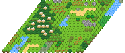
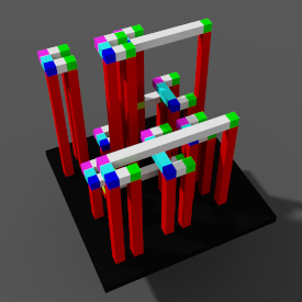
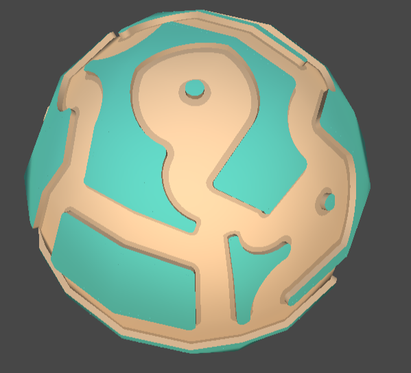
One obvious change is there’s no requirement to use square grids. WFC works just as well on hex grids, in 3d, or more unusual sufaces.

We can also introduce additional constraints, and fix particular tiles, or create “modules” which are tiles that span multiple cells.

Adding extra constraints can be quite important from a practical point of view. Because WFC only constrains nearby tiles, it rarely generates large scale structures, which can give large levels a homogenous, unplanned look. The best results seem to come when you let WFC do the tile picking, but a different technique or constraint to ensure some large structure.

I go into some detail how ways to get the best out of WFC in my tips and tricks article.

Overlapped WFC

One extension that is particularly interesting is “overlapped” WFC. In the above examples above the main constraint was concerned with pairs of tiles that are adjacent. That is sufficient to ensure lines join up, and create simple structures like caves and rooms and so on. But it still loses a lot of information. If we want that, say, red tiles are always near blue tiles, but never directly adjacent, it is hard to express this in terms of adjacencies only.

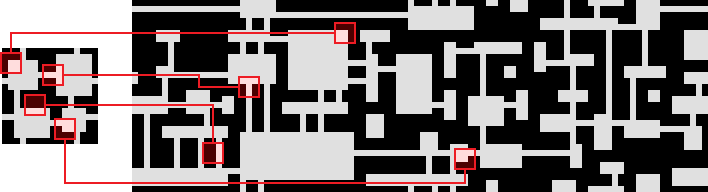
Enter overlapped WFC (also proposed by Maxim Gumin). We replace the adjacency constraints with a new constraint that affects multiple tiles at once: We require that each 3×3 group of cells in the output corresponds to a 3×3 group in a sample grid. The patterns that occur in the sample will get repeated over and over again in different variations in the ouput:

This constraint is vastly more sensitive than the “simple” adjacency constraints. And because it works from a given example, it’s very intuitive for artistic direction. So far, I haven’t seen nearly as much interest. That could be because it is harder to implement, slower to run or perhaps because it can sometimes be too good at reproducing the original sample, losing some of the organic feel.

Where to next?

Well, hopefully this tutorial has give you some idea how constraint solving and WFC works. Constraint solving is a large and active area of computer science, I barely touched on how it works here. You can find more information on Wikipedia.

While this sort of constraint solving dates to 2009, WFC itself is still relatively new. I recomend checking our r/proceduralgeneration, #wavefunctioncollapse and @exutumno, @osksta to get a show case of the latest projects people have been trying.

From me, you can read my WFC tips and tricks article, or experiment with my open source library or Unity asset for WFC. I’ve several other articles on procedural generation too. Let me know in the comments any feedback on the article, or what you’d like to hear about next.