I was browsing the Apache Arrow docs and spotted a term unfamiliar to me. Intrguied, I discovered that Compressed Sparse Fibers are a new technique for representing sparse tensors in memory. After reading up a bit, I thought I’d share with you what I’ve learnt. The technique is so new (well, 2015..) it is not mentioned on Wikipedia, and I found virtually nothing elsewhere. There’s a very limited number of ways to handle sparse data, so it’s always interesting to see a new one.
Don’t worry, I’d also never heard of a sparse tensor before, so I’m going to explain things right from the beginning, assuming you have a basic CS background, and don’t mind me going a little quickly.
Background Material
Let’s start with matrices. A matrix is essentially a 2d array of numbers, equipped with extra operations. They are at the heart of lot of mathematics, and have a great deal of deep properties, none of which I’m going to cover here.
As CSF is primarily a storage format, we don’t actually need to know how to use matrices or for what, we just want to know how to efficiently store things. We’ll just take the authors’ word for it that actually doing calculations on the stored data works out nicely (though there are some performance measurements in the paper describing it).
A tensor is the extension of matrices to multiple dimensions. That can get a bit fiddly mathematically, but again, for the purposes of this article, we’re just looking at storage, so a tensor is basically a multi-dimensional array. Numpy’s docs gives a fuller description of how they work. Tensors have become big news these days due to their near ubiquity in deep machine learning frameworks.
Finally, what about sparsity? Well, it turns out one of the most common use cases for multidimensional arrays is one where the vast majority of of the entries of the array are empty (equal to zero). Sparsity covers techniques that are optimized for this specific use case, avoiding storing all the empty data.
For example, you might want to consider Netflix’s database of user ratings. There’d be one row for every movie, and one column for every user, and we’d fill in values 1 to 5 in a cell each time a given user rates a given movie. But no one really watches that many movies, so most cells are empty. It would be a huge waste of memory to store the entire array. Of course, we can do better. Instead, we’d have a table of data with three columns: user, movie, rating. There would be one row per rating, and there is no storage cost for pairs of users and movies that have no rating.
It might seem odd to you to describe a database table, a common programming technique, as a compression method for storing a gigantic 2d array, but there are advantages to this line of thought. By considering it as an array, we can apply matrix operations to it. The insight that a form of Singular Value Decomposition could be applied to Netflix’s database became the basis for the victors of the Netflix Prize, an early ML competition for predicting what users would like what movies.
Sparsity is also used a lot in game development, for example when saving Minecraft levels, but I’ll have to discuss that another time.
Matrix Sparsity
When it comes to storing sparse matrices, there are only a handful of ways of doing it. That’s generally a good thing – most algorithms have to be hand written depending on the storage format, so more storage patterns means more pain when making and using libraries.
I’ll cover a few of the most common formats.
First up is just using a normal array, i.e. storing every value, even the zeros, consecutively in memory in a fixed order. This is called a dense array to disambiguate it from other sparse methods. Obviously, dense arrays don’t make any use of our assumption that most values are zero, so they can use lots of memory. But they still are often the best choice as they have the closest match to how modern hardware operates.
For example, the matrix
\[ \begin{pmatrix}
10 & 20 & 0 & 0 & 0 & 0 \\
0 & 30 & 0 & 40 & 0 & 0 \\
0 & 0 & 50 & 60 & 70 & 0 \\
0 & 0 & 0 & 0 & 0 & 80 \\
\end{pmatrix} \]
Would be stored in memory as a length 24 array
[ 10, 20,  0,  0,  0,  0,
   0, 30,  0, 40,  0,  0,
   0,  0, 50, 60, 70,  0,
   0,  0,  0,  0,  0, 80 ]
The next most common format is a co-ordinate list (COO). We’ve already seen how this works in the Netflix example above. We store one entry for each non-zero value, and that entry includes row index, column index and the value itself.
So our example matrix
\[ \begin{pmatrix}
10 & 20 & 0 & 0 & 0 & 0 \\
0 & 30 & 0 & 40 & 0 & 0 \\
0 & 0 & 50 & 60 & 70 & 0 \\
0 & 0 & 0 & 0 & 0 & 80 \\
\end{pmatrix} \]
would become
| Row | Column | Value |
|---|---|---|
| 0 | 0 | 10 |
| 0 | 1 | 20 |
| 1 | 1 | 30 |
| 1 | 3 | 40 |
| 2 | 2 | 50 |
| 2 | 3 | 60 |
| 2 | 4 | 70 |
| 3 | 5 | 80 |
Finally, a slightly more sophisticated format exists called Compressed Sparse Row (CSR).
CSR uses three separate arrays, values, col_indices and row_indprt. To fill them, we first get the COO entries for the sparse matrix, sorted by row, then column. values is filled non-zero values, in order. col_indices is filled the column index for each non zero value. Then the final array has size row_count+1. Each entry corresponds to a row in the original matrix, and indicates the first value in the value array that belongs to the row.
For example
\begin{pmatrix}
10 & 20 & 0 & 0 & 0 & 0 \\
0 & 30 & 0 & 40 & 0 & 0 \\
0 & 0 & 50 & 60 & 70 & 0 \\
0 & 0 & 0 & 0 & 0 & 80 \\
\end{pmatrix}
would become
    values      = [ 10, 20, 30, 40, 50, 60, 70, 80 ]
    col_indices = [  0,  1,  1,  3,  2,  3,  4,  5 ]
    row_indptr  = [  0,  2,  4,  7,  8 ]
To read values for a given row back out again, we first read a pair of values from the row indptr array, and then use those to slice the other two arrays. E.g. to read the third row, we’d find row_indptr[2] = 4 and row_indptr[3] = 7, which tells us that there are 3 values in that row, with columns col_indices[4], col_indices[5] and col_indices[6] and values values[4], values[5] and values[6].
In other words, compared with the COO format, it avoids repeating the row index over and over again – as the values are ordered, we know that all values in a given row will be consecutive. We can say that the row data hase been compressed. The column and value data is still uncompressed though – it takes up as much spaces as it did in the COO format.
There’s also the Compressed Sparse Column (CSC) which is exactly the same as CSR, just with rows and columns fixed.
I’ve skipped a few other formats, but they are either fairly trivial or specialized for particular uses.
Generalizing to tensors
Most of the above storage techniques generalize just as well to more dimensions. Suppose we have a n-dimensional array instead of a 2d one. Well, now instead of a row index and a column index required to identify a particular value, we now need n different indices. Or equivalently, we’d use a single n-tuple as the index.
COO works much as it did before. Instead of having 2 index arrays and one value array , we now have n index arrays and one value array.
A 4 dimensional COO dataset might look like
| i | j | k | l | Value |
|---|---|---|---|---|
| 1 | 1 | 1 | 2 | 1.0 |
| 1 | 1 | 1 | 3 | 2.0 |
| 1 | 2 | 1 | 1 | 3.0 |
| 1 | 2 | 1 | 3 | 4.0 |
| 1 | 2 | 2 | 1 | 5.0 |
| 2 | 2 | 2 | 1 | 6.0 |
| 2 | 2 | 2 | 3 | 7.0 |
| 2 | 2 | 2 | 2 | 8.0 |
CSR is a bit fiddlier. We’d now pick the first of the dimensions to be the compressed into a shorter array, then keep n-1 index arrays and one value array from COO.
We’d store the above data like so:
values   = [ 1.0, 2.0, 3.0, 4.0, 5.0, 6.0, 7.0, 8.0 ]
j        = [   1,   1,   2,   2,   2,   2,   2,   2 ]
k        = [   1,   1,   1,   1,   2,   2,   2   2 ]
l        = [   2,   3,   1,   3,   1,   1,   3,   2 ]
i indptr = [ 0, 0, 5, 8 ]
As you can see, CSR, is less beneficial in higher dimensions as it only compresses one of the dimensions.
Compressed Sparse Fibers
Ok, I think we’re finally ready to tackle how CSF works.
If we review how row compression worked, it was based on the idea that if we ordered the values by row, then by column, then we know that all the values for a given row are consecutive. So rather than storing repeat copies of the row index, we just need to know what slice of the value array belongs to each row.
Once we move to three dimensions, we can order the values by i, j, k (dimensions 1, 2 and 3). So it’ll still be true that all the values with a given i will be consecutive (as it was the first we sorted by). And if we filter to just a specific value of i, then all the values with a given j will be consecutive (as we’ve ordered by it second). And so on, if we had even more dimensions to work with.
So what we can do is use compression on the first dimension, then group each of the values by their first dimension index. Each value in that group is identified by it’s remaining n-1 indices, in other words it is itself a n-1 dimensional tensor.
In the 4d example above, we could split it on the first dimension to give two fibres. The i=1 subtensor:
| j | k | l | Value |
|---|---|---|---|
| 1 | 1 | 2 | 1.0 |
| 1 | 1 | 3 | 2.0 |
| 2 | 1 | 1 | 3.0 |
| 2 | 1 | 3 | 4.0 |
| 2 | 2 | 1 | 5.0 |
And the i=2 subtensor:
| j | k | l | Value |
|---|---|---|---|
| 2 | 1 | 1 | 6.0 |
| 2 | 1 | 3 | 7.0 |
| 2 | 2 | 2 | 8.0 |
Now we have n-1 dimension tensors, we can talk about how to store them. The natural approach is to recursively repeat the process – compress a dimension, group into subtensors, repeat. If the data is already sorted correctly, we don’t even need group, just find where the runs start and end.
The end result is a tree of index values, where each generation of the tree corresponds to one of the dimensions. Here’s a diagram showing how a 4 dimensional tensor could be compressed.
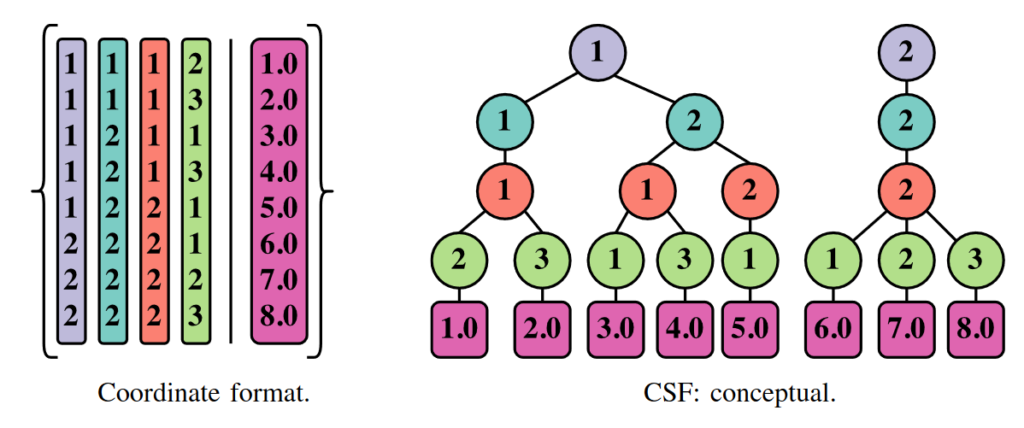
As you can see, some of the repetition of the original table has been eliminated. The earlier dimensions are compressed a lot, and the last dimension has no compression at all. But the net effect can be effective.
Each of the subtrees in the diagram correspond to a multidimensional slice of the original tensor. That makes it a convenient format for evaluating matrix algorithms on, as many of them also work by taking slices.
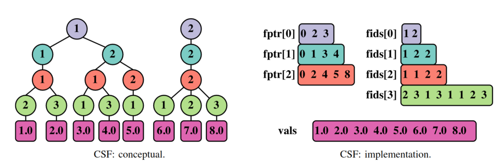
We don’t need literally store a tree structure though. Like CSR, the structure is amenable to being packed into arrays. Each dimension adds two arrays – one to indicate the what indices are present in that dimension, and one to show how to slice the next dimension.
The final cherry on top is to add a bit of flexibility to the system. Rather than always sorting the dimensions in a fixed order, we can actually pick which is most appropriate for our given tensor. You might want to pick a very narrow dimension as the first one to sort by, so that it gets the best compression. And you don’t have to compress all the dimensions, you can have some sparse, and some dense, and get the best of both worlds.
Another way I like to think about CSF is that we basically want to store a sorted set of n-tuples (the indices). One efficient way of doing so it to build a trie of the tuples of depth n, and store values in each leaf node.
Conclusion
So why did I find this so interesting, even though I don’t do anything with multidimensional sparse tensors, and probably never will?
To me, it’s the flexibility that CSF brings. By playing with the ordering and compression of dimensions, you can achieve a variety of effects. In 2d, it can be thought of as a general framework which is a superset of both CSR and CSC, and also interacts very nicely with COO and dense arrays.
Having one system that can cover all that ground will hopefully save future library writers from writing half a dozen copies of the same algorithm for different storage formats. But CSF is not the only contender for that spot – other techniques such as Generalized CSR might also work. We’ll have to see what the industry settles on.