Recently I’ve been looking at Mesh Welding algorithms.

Mesh Welding is when you have a a mesh, i.e. a collection of vertices, edges and faces, and you merge any vertices which are close enough together.

This is a common operation in procgen, as it’s often convenient to generate several things completely independently, then join them together afterwards. I’ve had to re-implement it several times.

I call it mesh welding, as that’s how I’ve encountered it, but really, the edges and faces of the mesh are irrelevant – all that matters is locating clusters of points that are near each other, the rest of the mesh just follows from that.

It’s an operation that is ok to be a bit sloppy, so I’m going to pick some merge rules that make things easy.

• when merging points, you can pick one arbitrarily to be the position of the result points. No need to average.
• points that are within distance \(r\) *must* eligible for merging, and points that are separated by \(R\) are not (unless there is some intervening points between the two). But distances between \(r\) and \(R\) are an arbitrary choice
• When all merges are done, there must be no points within distance \(r\) of each other.

To give you an idea what I mean, imagine a row of points, each separated by \(r\). It would be a perfectly acceptable weld to merge every odd numbered point into the next even number, leaving a row of half as many points each separated by \(2r\). Some other weld algorithms might weld such a line into a single point, but chasing connections like that usually makes for an unwieldy algorithm.

Naive Approach

Of course, we can implement welding by looping over every pair of points, and greedily merging them if they are close. But this is quadratic performance. We can do better by taking advantage of geometry of the problem.

Spatial Hashing

Spacial hashing is one of the easiest data structures for games and procgen. In other scenarios, it’s inflexibility makes it quite a poor choice, but in the context procedural generation, we don’t tend to run into hard cases where it would flop.

For simplicity, I’m going to consider points in 2d, but the principles extend to 3d.

The easiest way to employ spatial hashing is to divide the plane into square cells of size \(r\). We have a store which holds a value per cell, initially empty.

We then loop over the points and for each one:

• Find the cell that contains the point:
• Search the store for that cell and its 8 neighbors (i.e. including diagonals)
• If you found any point already in the store, merge the current point with the found one.
• Otherwise, store the point in the cell.

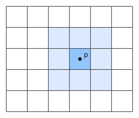
Or as pseudocode:

store = {}
for p in points:
  cell_x = floor(p.x / r)
  cell_y = floor(p.y / r)
  for dx in [-1, 0, 1]:
    for dy in [-1, 0, 1]:
      cell2_x = cell_x + dx
      cell2_y = cell_y + dy
      if (cell2_x, cell2_y) in store:
        merge(p, store[cell2_x, cell2_y)
        continue to next p
  store[cell_x, cell_y] = p 

I’m relying on my “loose” definition of welding. For other definitions, you need to store multiple points per cell, and track their positions, so you can be a bit more precise about distances. But either way, they are relying on the fact that the cell a point is in tells you a lot about the distances between points:

• If two points are in adjacent cells, then the distances between them is at most \(2r\).
• If two points are in non-adjacent cell, then the distanct between them is at least \(r\).

The same thing works in 3d, but you end up with 27 cells to check instead of 9, i.e. the 3x3x3 cube centered around the found cell.

You best make sure that the store is a *sparse* store, like a dictionary, though. \(r\) is typically very small, so the number of possible cells vastly out numbers the points you are analysing, and most cells will remain empty and unused.

Doing Better

This algorithm is already \(O(n)\), but the actual speed of it can be a bit disappointing. Checking the store at a given cell involves a dict lookup, and we are doing 9 (or 27) of them per point! We need to cut that down.

We can do a trade off. If we make the cells *larger* than \(r\) then we need to search fewer cells. But there would be more stuff in the cells. For example, suppose we made the cells \(100r\). Then any point that falls inside the \(98r \times 98r\) rectangle centered inside the cell would only need to search that one cell, as the point is further than \(r\) from any border of the cell. But that one cell is enormous, so we run the risk that many points that are not really near each other would all get lumped into that one cell.

So the tradeoff does depend quite a bit on the sparsity of your points.

The tradeoff I like is to pick cells that are size \(2r\). This admits a very neat hashing scheme that only searches 4 cells (8 in 3d), because the storage grid is offset by \(r\) from the search grid.

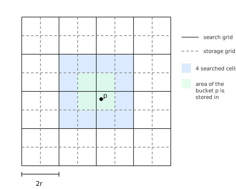
In pseudo code

store = {}
for p in points:
  cell_x = floor(p.x / 2 / r)
  cell_y = floor(p.y / 2 / r)
  for dx in [0, 1]:
    for dy in [0, 1]:
      cell2_x = cell_x + dx
      cell2_y = cell_y + dy
      if (cell2_x, cell2_y) in store:
        merge(p, store[cell2_x, cell2_y)
        continue to next p

  store_cell_x = floor(p.x / 2 / r + 0.5)
  store_cell_y = floor(p.y / 2 / r + 0.5)
  store[store_cell_x, store_cell_y] = p

To see why this works, imagine you are in the top left quadrant of a \(2r \cross 2r\) cell. Then the right neighbour of the cell is more than half the cell away, so any points in it are further than \(r\). There’s only four cells near enough – the current one, the one to the left, above, and diagonal.

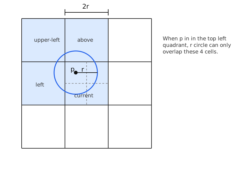
The rounding offset above essentially helps split cells into quadrants, as each quadrant of a cell with find a different value for store_cell.

But despite using only 4 searches, rather than 9, because the cells are larger, it’s less discriminating – it covers an area of \(16r^2\) vs the original \(9r^2\) (or 64 vs 27 for the 3d case). I still like it because the logic is simple – I think for any other size of cell, the number of lookups is variable and more fiddly to implement.

…that is, for square cells. You can actually employ a similar trick using hexagons and triangles. The store cell is done on a hexagonal grid with side length \(2r\). When searching, you first check which triangle you are on in the dual grid. Then you search the three hexagons that cover the triangle corners. This has even worse blow up than the 4 square search, as it covers \(\approx 31.8r^2\) area. But it’s neat.

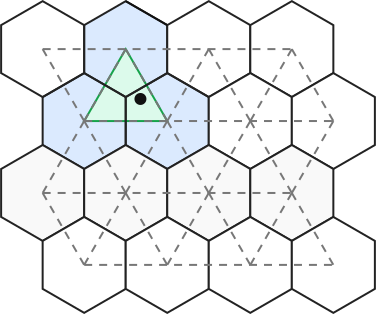
There’s a similar construction in 3d that only uses 4 lookups, using truncated octahedra instead of hexagons, but I think no one is going to do that in practice.

kd-trees

Of course, after implementing much of this in my library, it finally occurred to me to look up how blender does it. It uses a kd-tree which lets you quickly search for nearby points. This might be a bit slower in some cases, but it’s a much safer pick: The problem with spatial hashes is that they really work best when your points are roughly uniform, which there are no guarantees in a general purpose library.