One issue with 2d Marching Cubes (i.e. Marching Squres) that I glossed over in my original tutorial is the issue of ambiguity. Later I talk about how dual contouring avoids this problem. But it turns out there’s actually a well known, but little documented way of resolving those ambiguities called the Asymptotic Decider, which I’ll explain below.

The Problem

In Marching Cubes, you select which of 16 cases to use for a given cell, based on whether the 4 corners of that cell are solid or empty. But there were some cases where you could select two equally sensible choices.

For example, here’s two possible configurations for a single case:

The left configuration separates the two white corners from each other, while the right configuration separates the the black corners from each other.

In the the absence of futher information, there’s not much you can do here, and you might as well pick arbitrarily, which is exactly what I did in that tutorial.

The Solution

The point is, we often do have more information. Later in that same article, I assumed that you have numerical values associated with each vertex, with positive values for solid vertices, and negative for empty vertices. You can use these to shift around the output to give a better fit for the target.

If you have those numerical values, then the ambiguous cases are those where the top_left and bottom_right have both positive, and bottom_left and top_right are negative. Or visa versa.

In those cases, compute:

 Q = top_left * bottom_right - bottom_left * top_right

If Q is positive, use one of the possible configurations. If negative, use the other. That’s it!

The Explanation

If the top left vertex has a positive value, say 0.6, and the top left vertex has a negative value, say -0.3, then we can work out the place that crosses zero when doing linear interpolation.

If we use that point, rather than the midpoint, then we marching squares gives a much smoother approximation of our original surface, a property I called adaptivity.

So interpolation alone the top edge basically shows you how which parts of that edge are positive, and which parts are negative. Similar interpolation works along each of the sides.

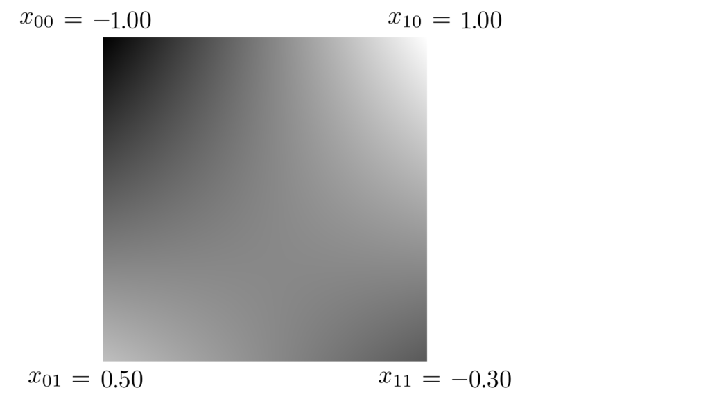
But in fact, we can use interpolation to think about the interior of the cell too. It’s a process called bilinear interpolation. It’s easiest to think of bilinear interpolation as interpolating horizontally along the top edge and bottom edges to get two points, then interpolating vertically between those points to get the final point.

That lets us fill in a numeric value for every point in the cell.

We can then analyse whether those points are above or below zero.

Then we just look at which corners are connected by a single block of color, and pick a marching squares case that matches that connectivity. Computing Q lets us easily determine which pair is connected. The original paper, The Asymptotic Decider: Resolving Ambiguities in Marching Cubes, Nielson & Hamann, goes into some details of the maths.

Here’s an animation putting the whole thing together.

What about 3d?

While 3d Marching Cubes is considerably more complex, there’s similar treatments. Most common is Marching Cubes 33 or Lewiner Marching cubes, which are each algorithms introduce a many more cases to marching cubes, using disambiguators like the the above to select between them.